on
Everyone ’ s a critic
Reinforcement Learning Saga — Part II:
From Q-learning to PPO
Code available here
In this article
- Deep Q-Networks
- Policy Gradient Methods
- Policy Gradient Theorem
- Baselines and the Advantage
- Advantage Actor-Critic
- Generalized Advantage Estimation
- Importance Sampling
- Trust Region Policy Optimization
- Proximal Policy Optimization
Abstract
Part I ended with Q-learning. Deep Q-Networks (DQN) extends it by replacing the table with a neural network, supported by experience replay and a frozen target network, but the policy is still obtained indirectly through a greedy maximization over discrete actions. We therefore move from learning values to learning the policy itself. Its objective is the expected return of the trajectories, and the policy gradient theorem makes that objective differentiable without requiring the unknown dynamics of the environment. A baseline changes the learning signal from the absolute return to whether the action performed better or worse than expected: its advantage. To use the advantage, the state-value function is needed, so a critic learns it with TD: we obtained Advantage Actor-Critic (A$2$C). The one step estimate is biased, Monte Carlo is noisy: Generalized Advantage Estimation (GAE) combines several horizons to balance.
The direction of the update is clear, but each batch of on-policy data is discarded after one step. Importance sampling makes that data reusable by correcting for the change in action probabilities, although the correction is reliable only while the new policy remains close to the old. TRPO enforces this with a trust-region constraint, but requires expensive second-order optimization. PPO reaches the same practical goal with a clipped, first-order objective.
Deep Q-Networks
In Part I, we terminated with Q-learning: a table with one entry $Q(s,a)$ per state-action pair, updated from experience, with the policy implicitly defined on top (act greedily, explore occasionally). A limitation of this approach is the table itself: it requires one entry per state, and outside of grid worlds the state space explodes. A game screen of $84 \times 84$ grayscale pixels with $256$ intensity levels has $256^{84 \times 84}$ possible states: enumerating them is out of question, and even if we could, every entry is learned in isolation: updating one state teaches nothing about the millions of nearly identical states never visited, because a table has no notion of two states being similar.
The natural fix is to replace the table with a function approximator. Deep Q-Networks (DQN) uses a convolutional network $Q_\theta(s,a)$, with parameters $\theta$, that reads the state (e.g. the game screen) and outputs one value per action, so that states never seen before still get sensible values because they resemble states that were. The learning objective remains the same: move the current Q-value estimate toward the standard TD target. In tabular Q-learning we had:
\[Q_\pi(s_t,a_t) \leftarrow Q_\pi(s_t,a_t) +\alpha\,\Big( \underbrace{ r_{t+1} + \gamma\, \max_{a'} Q_\pi(s_{t+1},a') }_{\text{TD target}} - \underbrace{ Q_\pi(s_t,a_t)\vphantom{r_{t+1} + \gamma \max_{a'} Q_\pi(s_{t+1},a')} }_{\substack{\text{current}\\\text{estimate}}} \Big)\]With DQN, since there is no table entry to overwrite, the update is performed by adjusting the network parameters $\theta$. This is done by minimizing the loss function $L(\theta)$:
\[L(\theta) = \mathbb{E}\Big[\big(\underbrace{r + \gamma\,\max_{a'} Q_\theta(s', a')\\[4pt]}_{\text{TD target}} - \underbrace{ Q_\theta(s,a)\vphantom{r_{t+1} + \gamma \max_{a'} Q_\pi(s_{t+1},a')} }_{\substack{\text{current}\\\text{estimate}}}\big)^2\Big]\]Done naively, this is unstable. Training a neural network is a supervised learning procedure, and plugging Q-learning into it violates its assumptions in two distinct ways.
-
Data is not i.i.d.. For example, in a gameplay, consecutive frames are strongly correlated. Gradient descent (used to minimize $L(\theta)$) expects shuffled data and instead receives a stream where each minibatch is a biased snapshot of one small corner of the game.
-
The target moves with the network. The TD target is computed from the same network that is being trained. Every gradient step drags the target along with the prediction, and the network ends up chasing itself.
DQN addresses these two issues with a couple of mechanisms.
-
Experience replay. Every experience $(s,a,r,s’)$ is stored in a large replay buffer. Each gradient step samples a random minibatch from this buffer. Random sampling destroys the temporal correlations in a single gameplay trajectory, so each minibatch becomes a much better approximation of an i.i.d. dataset.
-
Target network. Instead of computing the target with the network that is being trained, DQN keeps a second network, $Q_{\theta^-}$, whose parameters are held fixed while the main network $Q_\theta$ learns. During many consecutive gradient steps, the prediction changes but the target does not, turning the optimization into an ordinary regression problem with temporarily fixed labels. Only every $C$ steps $Q_{\theta^-}$ is refreshed by copying $Q_\theta$. Therefore, instead of chasing a target that moves after every update, the network learns toward a stable objective before the target is moved again.
- Initialize Q-network with random weights $\theta$
- Initialize target network with weights $\theta^- \leftarrow \theta$
- Initialize replay memory $\mathcal{D}$
- Initialize hyperparameters
- $\gamma\;$ discount factor
- $\varepsilon\;$ exploration rate
- $\alpha\;$ learning rate
- $B\;$ minibatch size
- $C\;$ target update frequency
- Repeat until convergence:
- Start the agent at state $s_0$
- Repeat until $s$ is terminal:
- Take action $a = \arg\max_{a} Q_\theta(s,a)$ ($\varepsilon$-greedy)
- Observe reward $r$ and next state $s'$, store transition $(s,a,r,s')$ in $\mathcal{D}$
- Sample a random minibatch of $B$ transitions $(s_i,a_i,r_i,s'_i)$ from $\mathcal{D}$
- Compute the TD target for each transition:
$$y_i =r_i + \gamma\, \textstyle{\max_{a'}}\, Q_{\theta^-}(s'_i,a')$$
- Compute the loss over all the $B$ transitions:$$L(\theta)= \textstyle{\frac{1}{B}\sum_{i=1}^{B}}\left(y_i - Q_\theta(s_i,a_i)\right)^2$$
- Update $Q_\theta$ parameters by gradient descent: $\theta\leftarrow\theta-\alpha\nabla_\theta L(\theta)$
- Every $C$ steps, update the target network: $\theta^- \leftarrow \theta$
- Move to the next state: $s \leftarrow s'$
- Decay $\alpha$ and $\varepsilon$
- Return optimal $Q_\theta$ and derived optimal policy $\pi^*$
DQN achieved human-level performance on Atari games, using only game screens as input. However, DQN is still indirect: it learns action values, and then a policy is derived by acting greedily. The next step is to make the policy itself a first-class object, something that can be represented, optimized, and improved directly.
Policy Gradient Methods
In value methods, the policy exists only through the values, as $\pi(s) = \arg\max_a Q_\theta(s,a)$. This works well when the actions are few and discrete, but it has some limitations that no amount of network capacity can fix.
-
The derived policy is deterministic. It always selects the same action in the same state. Exploration can be added with an $\varepsilon$-greedy rule, but it is not learned directly.
-
The maximization assumes a manageable action space. Both Q-learning and DQN require computing $\max_{a}Q(s,a)$. This is straightforward when there are few actions, but not when actions are continuous. Finding the best steering angle, for example, would require solving an optimization problem at every time step.
-
The values are an intermediate representation. The final objective is to learn how the agent should behave, but value methods first estimate the return of every action and only then derive the behavior. Errors in the estimates can change the selected action.
Policy methods remove the indirection by representing the policy itself as a parametrized function $\pi_\theta(a|s)$, with parameters $\theta$, typically the weights of a neural network. Given a state $s$, the network directly defines a probability distribution over actions: for a discrete action space this can be a softmax distribution over the available actions, for a continuous action space this can instead define the parameters of a distribution such as a Gaussian.
The problem has changed: in value-based learning $Q_\theta$ is adjusted so that its predictions satisfy the Bellman equation, in policy-based learning we adjust $\theta$ so that the actions sampled from $\pi_\theta$ lead to higher returns. Value functions will reappear later, but as a tool for evaluating and improving the policy, rather than as the final object being learned.
To optimize the policy, we first need a scalar measure of its performance. A trajectory $\tau$ is one complete sequence generated by following $\pi_\theta$.
\[\tau = (s_0,a_0,r_1,s_1,a_1,r_2,\,..\, ,s_T)\]Its discounted return $G(\tau)$ is the sum of all rewards obtained from the start until the episode conclusion, at time $T$, multiplied by the discount factor $\gamma$.
\[G(\tau) =r_{1} + \gamma\,r_{2} + \gamma^2\,r_{3} + \;..\; + \gamma^{T-1}\,r_{T} = \sum_{t=0}^{T-1}\gamma^t\, r_{t+1}\]The policy objective $J(\theta)$ is the expected return over all trajectories $\tau$ that can be generated by the current policy $\pi_\theta$. The goal is to find the parameters $\theta$ that maximize $J(\theta)$.
\[\begin{gathered} J(\theta) = \mathbb{E}_{\tau \sim \pi_\theta}\!\left[G(\tau)\right] = \sum_{\tau} p_\theta(\tau)\,G(\tau) \\[0pt] \big(\text{or} \int p_\theta(\tau)\,G(\tau)\,d\tau \, \text{ for continuous trajectories} \big) \end{gathered}\]Since the policy is differentiable, we would like to improve it through gradient ascent:
\[\theta \leftarrow \theta + \alpha \, \nabla_\theta J(\theta)\]where $\alpha$ is the learning rate. The difficulty is that $J(\theta)$ depends on $\theta$ through the probability of the sampled trajectories, $p_\theta(\tau)$. The probability of a trajectory under $\pi_\theta$ is:
\[p_\theta(\tau) = p(s_0)\, \prod_{t=0}^{T-1} \pi_\theta(a_t\,|\,s_t)\; p(s_{t+1}\,|\,s_t, a_t)\]This expression contains terms that we control, the policy $\pi_\theta$, and terms that belong to the environment, the initial-state distribution $p(s_0)$ and the transition probabilities $p(s_{t+1}|s_t,a_t)$. Since these dynamics are generally unknown, computing $\nabla_\theta J(\theta)$ appears to require a model of the environment. The policy gradient theorem shows that it does not.
Policy Gradient Theorem
The solution relies on the log-derivative trick. For any function $f$ parametrized by $\theta$:
\[\nabla_\theta f_\theta = f_\theta \,\nabla_\theta \log f_\theta\]which follows from the chain rule applied to $\nabla_\theta \log f_\theta = \smash{\frac{\nabla_\theta f_\theta}{f_\theta}}$. Let us now apply the trick to the gradient of the policy objective:
\[\begin{align} \nabla_\theta J(\theta) &= \nabla_\theta \textstyle\sum_{\tau} p_\theta(\tau)\,G(\tau)\\[2pt] &= \textstyle\sum_{\tau} \nabla_\theta \big(\,p_\theta(\tau)\,G(\tau)\big)\\[2pt] &= \textstyle\sum_{\tau} G(\tau)\,\nabla_\theta\, p_\theta(\tau)\\[-4pt] &\overset{1}{=} \textstyle\sum_{\tau} p_\theta(\tau)\,\nabla_\theta \log p_\theta(\tau)\,G(\tau)\\[2pt] &= \textstyle\mathbb{E}_{\tau\sim\pi_\theta}\!\left[\nabla_\theta \log p_\theta(\tau)\,G(\tau)\right] \end{align}\]$^1$ Log-derivative trick applied to $\nabla_\theta\,p_\theta(\tau)$.
Next, we expand $\log p_\theta(\tau)$ using the expression of the trajectory probability:
\[\log p_\theta(\tau) = \log p(s_0) + \sum_{t} \log \pi_\theta(a_t|s_t) + \sum_{t} \log p(s_{t+1}|s_t,a_t)\]The initial distribution and the transition probabilities do not depend on $\theta$, so their gradient with respect to $\theta$ is zero and they simply vanish:
\[\nabla_\theta \log p_\theta(\tau) = \sum_{t} \nabla_\theta \log \pi_\theta(a_t|s_t)\]All the terms belonging to the environment disappeared: even though the objective depends on the unknown dynamics, its gradient does not. To improve the policy, we only need the gradient of the log-policy, evaluated on trajectories sampled by acting in the environment:
\[\nabla_\theta J(\theta) = \mathbb{E}_{\tau\sim\pi_\theta}\Big[\sum_t \nabla_\theta \log \pi_\theta(a_t|s_t)\; G(\tau)\Big]\]One further refinement is possible. By causality, the action taken at time $t$ cannot influence the rewards collected before $t$. Each term of the sum can therefore be weighted by the return from $t$ onward, $G_t$, rather than by the return of the whole trajectory.
Policy gradient theorem $$ \nabla_\theta J(\theta) = \mathbb{E}_{\tau\sim\pi_\theta}\Big[\smash{\sum_t} \nabla_\theta \log \pi_\theta(a_t|s_t)\; G_t \,\Big] $$
The intuition behind the formula is the following. The term $\nabla_\theta \log \pi_\theta(a_t|s_t)$ is the direction in parameter space that increases the probability of taking action $a_t$ in state $s_t$. That direction is weighted by the return $G_t$: actions followed by high returns become more likely, actions followed by low (or negative) returns become less likely. The policy gradient is reinforcement in its most literal form: behavior is repeated in proportion to how well it worked.
The vanilla policy gradient is unbiased, but it has the weaknesses of Monte Carlo methods. Updates can only happen at episode boundaries, and single-sample returns are extremely noisy: the same action in the same state can be followed by very different returns, depending on what happens later in the episode. High variance in the gradient translates into slow and unstable learning. For this reason, the raw recipe is rarely used as is.
Baselines and the Advantage
A first source of variance lies in the returns themselves: their scale is arbitrary. Suppose every return in an environment is between $90$ and $100$. Then every action becomes more likely after each update, only with slightly different intensities, and the policy improves solely through the small differences between these pushes. What should matter is not whether the return was large in absolute terms, but whether it was larger than expected.
This motivates subtracting a baseline $b(s_t)$ from the return:
\[\nabla_\theta J(\theta) = \mathbb{E}_{\tau\sim\pi_\theta}\Big[\sum_t\nabla_\theta \log \pi_\theta(a_t|s_t)\, \big(G_t - b(s_t)\big)\Big]\]Any baseline that depends only on the state (not on the action) leaves the gradient unbiased. To prove it, let us first pull the $\textstyle\sum_t$ outside the expectation and focus on each component of the inner expression.
\[\mathbb{E}_{\tau\sim\pi_\theta}\Big[\sum_t\nabla_\theta \log \pi_\theta(a_t|s_t)\, b(s_t)\Big] = \sum_t \mathbb{E}_{\tau\sim\pi_\theta}\Big[\nabla_\theta \log \pi_\theta(a_t|s_t)\, b(s_t)\Big]\]The goal is to prove that the term is zero for each timestep separately.
\[\begin{align} \mathbb{E}_{\tau\sim\pi_\theta}[\nabla_\theta \log \pi_\theta(a_t|s_t)\, b(s_t)] &\overset{1}{=} \textstyle \sum_\tau p_\theta(\tau) \,\nabla_\theta \log\pi_\theta(a_t|s_t)\,b(s_t)\\[-4pt] &\overset{2}{=} \textstyle \sum_s p_\theta(s_t) \sum_a \pi_\theta(a_t|s_t) \,\nabla_\theta \log\pi_\theta(a_t|s_t)\,b(s_t)\\[2pt] &= \textstyle \sum_s p_\theta(s_t)\, b(s_t)\sum_a \pi_\theta(a_t|s_t) \,\nabla_\theta \log\pi_\theta(a_t|s_t)\\[-4pt] &\overset{3}{=} \textstyle \sum_s p_\theta(s_t)\, b(s_t)\sum_a \nabla_\theta\, \pi_\theta(a_t|s_t)\\[2pt] &= \textstyle \sum_s p_\theta(s_t)\, b(s_t) \,\nabla_\theta\sum_a \pi_\theta(a_t|s_t)\\[2pt] &= \textstyle \sum_s p_\theta(s_t)\, b(s_t) \,\nabla_\theta \,1\\[-4pt] &\overset{4}{=} 0 \end{align}\]$^1$ The expectation is over full trajectories, we are averaging over all possible episodes $\sim\pi_\theta$.
$^2$ Instead of thinking about complete trajectories, for a fixed $t$ we consider the probability of reaching a state and then selecting an action: $\textstyle \sum_\tau p_\theta(\tau)(\cdot) = \sum_s p_\theta(s_t=s) \sum_a \pi_\theta(a|s)(\cdot)$.
$^3$ Log-derivative trick applied to $\pi_\theta(a_t|s_t) \,\nabla_\theta \log\pi_\theta(a_t|s_t)$.
$^4$ $\nabla_\theta\,1 = 0$, derivative of a constant.
The baseline proof tells us that we are free to subtract any function that depends on the state. The goal is to choose a baseline that removes the part of the return that is not useful for deciding between actions. The natural choice is the expected return from the state, i.e. the state-value function $V_\pi(s)$.
\[b(s) = V_{\pi}(s) = \mathbb{E}_{\pi}[G_t\,|\,s_t=s]\]$G_t - V_\pi(s_t)$ measures how much better or worse the outcome was compared with what was expected from the state $s_t$. However, $G_t$ is a single sampled return: if we visit the same state and take the same action multiple times, the return can differ due to different future actions. $G_t$ is a noisy estimate of the expected value of taking that action. The expected return after taking action $a$ in state $s$ is the action-value function $Q_\pi(s,a)$.
\[Q_{\pi}(s,a) = \mathbb{E}_{\pi}[G_t\,|\,s_t=s, a_t=a]\]To obtain the true learning signal for the action $a_t$ in state $s_t$, we should average over all possible futures that can follow the action, rather than relying on the single future that happened to be sampled. This replaces the noisy Monte Carlo quantity $G_t - V_\pi(s_t)$ with its expectation $Q_\pi(s_t,a_t) - V_\pi(s_t)$. This difference is called the advantage function $A_\pi(s,a)$.
\[A_\pi(s,a) = Q_\pi(s,a) - V_\pi(s)\]The advantage measures how much better the action $a$ is compared to the average action in state $s$ under the policy $\pi$: if $A_\pi(s,a) > 0$ the action is better than what the policy would do on average and its probability should increase, if $A_\pi(s,a)<0$, it should become less likely. Conceptually, it is the advantage that drives learning, not the sampled return. In practice, vanilla policy gradient methods do not know the true advantage, so they approximate it with $G_t - V_\pi(s_t)$. The policy gradient can therefore be written in its ideal form as:
\[\nabla_\theta J(\theta)=\mathbb{E}_{\tau\sim\pi_\theta}\!\Big[ \smash{\sum_t} \nabla_\theta\log\pi_\theta(a_t|s_t)\, A_\pi(s_t,a_t) \Big]\]Advantage Actor-Critic
The Monte Carlo estimate of the advantage, $G_t - V_\pi(s_t)$, has the usual drawbacks of Monte Carlo methods: the agent must wait until the episode finishes before computing $G_t$, and the sampled return has high variance because it includes all the randomness of the future. In Part I, temporal difference learning provided an alternative way to estimate value functions by bootstrapping from the current value estimates instead of waiting for the full return. The same idea can be applied here: replace the complete return by the one step target
\[G_t \quad\longrightarrow\quad r_{t+1} + \gamma V_\pi(s_{t+1})\]The advantage can now be estimated in two ways:
\[\begin{aligned} \hat A_t^{MC} &=G_t-V_\pi(s_t)\\[0pt] \hat A_t^{TD} &= r_{t+1}+\gamma\,V_\pi(s_{t+1})-V_\pi(s_t) = \delta_t \end{aligned}\]\(\hat{A}_t^{TD}\) is exactly the one step temporal difference error $\delta_t$ that we have already encountered. Why is the TD error an approximation of the advantage? The value function $V_\pi(s_t)$ predicts the expected return from the current state under the current policy. After taking action $a_t$, the agent observes one sample of this return, $r_{t+1} + \gamma\,V_\pi(s_{t+1})$. The TD error compares this sample with the prediction. A positive TD error means the observed transition was better than the value function predicted, while a negative TD error means it was worse. The TD error therefore acts as an online estimate of the advantage. Although any single TD error is noisy, its conditional expectation equals to the advantage, making it a suitable signal for increasing or decreasing the probability of the selected action.
\[\begin{align} \mathbb{E}[\delta_t \,|\, s_t, a_t] &= \mathbb{E}[r_{t+1} + \gamma\, V_\pi(s_{t+1}) - V_\pi(s_t) \,|\, s_t, a_t]\\[-4pt] &\overset{1}{=} \mathbb{E}[r_{t+1} + \gamma\, V_\pi(s_{t+1}) \,|\, s_t, a_t] - V_\pi(s_t)\\[-4pt] &\overset{2}{=} \mathbb{E}[G_t \,|\, s_t, a_t] - V_\pi(s_t)\\[2pt] &=Q_\pi(s_t, a_t) - V_\pi(s_t)\\[2pt] &= A_\pi(s_t, a_t) \end{align}\]$^1$ Once $s_t$ is given, $V_\pi(s_t)$ is a constant and can be moved outside the expectation.
$^2$ Proven in Part I’s proof of Bellman equation for $Q_\pi(s,a)$.
There is one remaining issue: $V_\pi$ is unknown. Advantage Actor-Critic (A$2$C) methods solve it by learning the value function alongside the policy, keeping two parametrized components:
- the actor $\pi_\theta(a|s)$ (policy), which selects actions and is updated with the policy gradient
- the critic $V_w(s)$, an estimate of the state-value function, updated with TD learning
At each transition, the critic provides the one step ($\hspace{1pt}^{(1)}$) advantage estimate:
\[\smash{\hat{A}}_t^{(1)} = \delta_t = r_{t+1} + \gamma\,V_w(s_{t+1}) - V_w(s_t)\]The actor uses this estimate to update the policy through gradient ascent. In the formulation, the latest version of the policy gradient $\nabla_\theta J(\theta)$ was the one including $A_\pi$, which we are now approximating with $\smash{\hat{A}_t^{(1)}} = \delta_t$.
\[\begin{align} \theta &\leftarrow \theta + \alpha_\theta\,\nabla_\theta J(\theta)\\[2pt] &\leftarrow \theta + \alpha_\theta\, \mathbb{E}_{\tau\sim\pi_\theta} [\textstyle \sum_t \nabla_\theta\log\pi_\theta(a_t|s_t)\, A_\pi(s_t,a_t) ]\\[2pt] &\leftarrow \theta + \alpha_\theta\, \mathbb{E}_{\tau\sim\pi_\theta} [\textstyle \sum_t \nabla_\theta\log\pi_\theta(a_t|s_t)\, \delta_t]\\[2pt] \end{align}\]The expectation over trajectories and the sum over timesteps describe the ideal update. In practice, however, A$2$C estimates the gradient from each sampled transition:
\[\theta \leftarrow \theta + \alpha_\theta\, \nabla_\theta \log \pi_\theta(a_t|s_t)\, \delta_t\]Over many transitions, these incremental updates approximate the original policy gradient.
The critic has a different objective. Unlike the actor, it does not try to maximize the expected return $J(\theta)$, it tries to minimize the value prediction error, so it uses gradient descent.
\[w \leftarrow w - \alpha_w \,\nabla_w L(w)\]To define the loss function $L(w)$, let us recap that the critic is a function $V_w(s)$ that answers to “given that I am in state $s$, how much total reward should I expect in the future?”. So the critic is estimating $V_\pi(s)$. The ideal supervised learning objective would be:
\[L(w) = \textstyle\frac{1}{2} (V_\pi(s_t) - V_w(s_t))^2\]but since $V_\pi(s_t)$ is unknown, we use the current TD target estimate, which says that the value of the current state is the immediate reward plus the discounted value of the next state.
\[L(w) = {\textstyle\frac{1}{2}} \big( \, \underbrace{ r_{t+1} + \gamma\,V_w(s_{t+1}) }_{\text{TD target}} - V_w(s_t)\big)^2 = \textstyle\frac{1}{2} \delta_t^2\]Therefore:
\[\begin{align} \nabla_w L(w) &= \textstyle{\frac{1}{2}} \nabla_w (r_{t+1} + \gamma\,V_w(s_{t+1}) - V_w(s_t))^2\\[2pt] &= (r_{t+1} + \gamma\,V_w(s_{t+1}) - V_w(s_t)) \,\nabla_w (r_{t+1} + \gamma\,V_w(s_{t+1}) - V_w(s_t))\\[2pt] &= \delta_t \, ( \nabla_w(r_{t+1} + \gamma\,V_w(s_{t+1})) - \nabla_w V_w(s_t))\\[-4pt] &\overset{1}{=} - \delta_t \,\nabla_w V_w(s_t) \end{align}\]$^1$ The component $r_{t+1} + \gamma\,V_w(s_{t+1})$ is treated as a constant target during the critic update, so its gradient is zero. This is called the semi-gradient method.
The critic update takes the form of:
\[w \leftarrow w + \alpha_w \,\nabla_w V_w (s_t) \, \delta_t\]The same error then drives both components: it tells the actor how to change the probability of the action it has just taken, and it tells the critic how to correct its estimate of the state it has just evaluated. Both are updated after every step.
- Initialize actor parameters $\theta$ and critic parameters $w$
- Initialize learning rates $\alpha_\theta$, $\alpha_w$, discount $\gamma$
- Repeat until convergence:
- Start the agent at state $s_0$
- Repeat until $s$ is terminal:
- Take action $a \sim \pi_\theta(\cdot\,|\,s)$, observe reward $r$ and next state $s'$
- Compute the TD error: $\delta = r + \gamma\, V_w(s') - V_w(s)$
- Update the actor: $\theta \leftarrow \theta + \alpha_\theta\, \delta\, \nabla_\theta \log \pi_\theta(a|s)$
- Update the critic: $w \leftarrow w + \alpha_w\, \delta\, \nabla_w V_w(s)$
- Move to the next state: $s \leftarrow s'$
- Return the learned policy $\pi_\theta$
Compared with the vanilla policy gradient, the variance drops substantially, since one noisy full return is replaced by one observed reward plus a learned estimate, and learning no longer waits for episode boundaries. The price is the bias: the critic is only an approximation, and bootstrapping on a wrong estimate steers the actor in the wrong direction. This is the Monte Carlo versus TD trade-off of Part I resurfacing one level up, where it applied to value estimates and now applies to policy updates.
To make things clear, let us go back to the example of Part I. Two states \(S = \{\text{low}, \text{high}\}\), two available actions \(A = \{x,y\}\), and the generated episode was:
\[(\text{low}, x) \xrightarrow{+1} (\text{high}, y) \xrightarrow{+2} (\text{low}, x) \xrightarrow{+3} \text{ terminal}\]The critic is a table with one value per state, which is the simplest possible form of $V_w$: the parameters are the entries themselves, $V_w(s) = w_s$, and no state shares anything with the others. Its gradient $\nabla_w V_w(s_t)$ is then $1$ for the state being evaluated and $0$ for all the others, so every other entry is multiplied by zero and stays where it is. The actor holds one preference parameter $\theta_{s,a}$ per state-action pair, turned into probabilities by a softmax:
\[\pi_\theta(a|s) = \frac{e^{\theta_{s,a}}}{\sum_{a'} e^{\theta_{s,a'}}}\, \qquad \nabla_{\theta_{s,a}} \log \pi_\theta(a|s) = 1 - \pi_\theta(a|s)\]The gradient on the right is the one of the action that was taken, but a single step moves both preferences of the state. With two actions, $\pi_\theta(y|s) = 1 - \pi_\theta(x|s)$: whatever $\theta_{s,x}$ gains, $\theta_{s,y}$ loses. Only the difference between the two preferences reaches the softmax, so that difference moves twice as far as either parameter on its own. Starting from zero, this keeps $\theta_{s,y} = -\theta_{s,x}$ at every step, and the probability of $x$ is:
\[\pi_\theta(x|s) = \frac{e^{\theta_{s,x}}}{e^{\theta_{s,x}} + e^{-\theta_{s,x}}}\]Below, only the preference of the action taken is written out, the other one mirrors it.
Everything is initialized to zero, so at the beginning both actions are equally likely in both states, $\pi_\theta(x|s) = \pi_\theta(y|s) = 0.5$, and both state values are $V_w(\text{low}) = V_w(\text{high}) = 0$. Let us consider $\alpha_\theta = 0.1$ for the actor, $\alpha_w = 0.5$ for the critic, and again for simplicity $\gamma = 1$.
\(\begin{align}
\quad\,\mathrel{\raise 1pt\hbox{$\scriptsize\bullet$}}
\normalsize\,\, t=0: \quad &\delta_0 = r_1 + \gamma\,V_w(\text{high}) - V_w(\text{low}) = 1 + 0 - 0 = 1\\[2pt]
&V_w(\text{low}) \leftarrow V_w(\text{low}) + \alpha_w\,\delta_0 = 0 + 0.5 \cdot 1 = 0.5\\[0pt]
&\theta_{\text{low},x} \leftarrow \theta_{\text{low},x} + \alpha_\theta\,\delta_0\,\big(1 - \pi_\theta(x|\text{low})\big) = 0 + 0.1 \cdot 1 \cdot 0.5 = 0.05
\end{align}\)
\(\begin{align}
\\[-20pt]\quad\,\mathrel{\raise 1pt\hbox{$\scriptsize\bullet$}}
\normalsize\,\, t=1: \quad &\delta_1 = r_2 + \gamma\,V_w(\text{low}) - V_w(\text{high}) = 2 + 0.5 - 0 = 2.5\\[2pt]
&V_w(\text{high}) \leftarrow V_w(\text{high}) + \alpha_w\,\delta_1 = 0 + 0.5 \cdot 2.5 = 1.25\\[0pt]
&\theta_{\text{high},y} \leftarrow \theta_{\text{high},y} + \alpha_\theta\,\delta_1\,\big(1 - \pi_\theta(y|\text{high})\big) = 0 + 0.1 \cdot 2.5 \cdot 0.5 = 0.125
\end{align}\)
\(\begin{align}
\\[-20pt]\quad\,\mathrel{\raise 1pt\hbox{$\scriptsize\bullet$}}
\normalsize\,\, t=2: \quad &\delta_2 = r_3 + \gamma\,V_w(\text{terminal}) - V_w(\text{low}) = 3 + 0 - 0.5 = 2.5\\[2pt]
&V_w(\text{low}) \leftarrow V_w(\text{low}) + \alpha_w\,\delta_2 = 0.5 + 0.5 \cdot 2.5 = 1.75\\[0pt]
&\theta_{\text{low},x} \leftarrow \theta_{\text{low},x} + \alpha_\theta\,\delta_2\,\big(1 - \pi_\theta(x|\text{low})\big) = 0.05 + 0.1 \cdot 2.5 \cdot (1 - 0.525) \approx 0.169
\end{align}\)
In the last step, $\pi_\theta(x|\text{low})$ is no longer $0.5$ but $0.525$, because the preference of $x$ in $\text{low}$ had already been increased to $0.05$ at $t=0$, while that of $y$ has been lowered to $-0.05$. After the episode, $\pi_\theta(x|\text{low}) \approx 0.58$: the actor has become more inclined to take $x$ in $\text{low}$, without ever computing a return.
Two observations. First, the values of the critic are exactly the ones obtained by TD($0$) in Part I, $0.5$, $1.25$ and $1.75$: the critic is doing nothing more than the value estimation of Part I, while the actor rides on the same errors. Second, all three TD errors are positive, so all three actions taken became more likely, including $x$ in $\text{low}$ at $t=2$. Monte Carlo would have disagreed on that one: using Part I’s estimate $V_\pi(\text{low}) = 4.5$, the weight of that action would have been $G_2 - V_\pi(\text{low}) = 3 - 4.5 = -1.5$, making $x$ less likely. The disagreement is the bias described. The critic starts pessimistic (all values at zero), so every observed transition looks better than predicted. As the critic gets closer to $V_\pi$, its errors become centered on the true advantage and the two signals agree.
Generalized Advantage Estimation
At this point we face a known dilemma: the one step TD error has low variance but is biased by the critic, while the full Monte Carlo return minus the baseline is unbiased but has high variance. TD($n$) resolved this tension for value functions by looking $n$ steps ahead before bootstrapping, the same construction works for advantages:
\[\hat{A}_t^{(n)} = \underbrace{r_{t+1} + \gamma\, r_{t+2} + \,..\, + \gamma^{n-1}\, r_{t+n} + \gamma^n\, V_\pi(s_{t+n})\\[4pt]}_{n\text{-step return}} - V_\pi(s_t)\]with \(\smash{\hat{A}_t^{(1)}} = \delta_t\) at one extreme and Monte Carlo at the other. Committing to a single fixed $n$, however, is not optimal. There is no reason why the best horizon should be the same in every state and at every stage of training. More importantly, a single $n$ ties each estimate to a single bootstrap point, the value \(V(s_{t+n})\): if the critic happens to be wrong, the advantage at that timestep inherits the error in full.
Generalized Advantage Estimation (GAE) avoids the choice by averaging over all horizons at once with weights that decay geometrically in $n$.
\[\hat{A}_t^{\,GAE \,(\gamma,\,\lambda)} = (1-\lambda)\big(\hat{A}_t^{(1)} + \lambda\hat{A}_t^{(2)} + \lambda^2\hat{A}_t^{(3)} + \,..\,\big) = (1-\lambda)\sum_{n=1}^{\infty}\lambda^{n-1}\hat{A}_t^{(n)}\]Given that $\textstyle\sum_{n\geq1} \lambda^{n-1} = \frac{1}{1-\lambda}$, the factor $(1-\lambda)$ normalizes the weights to sum to one. The parameter $\lambda\in[0,1]$ controls how quickly the weights decay: when $\lambda$ is small almost all the weight is assigned to the shortest, most heavily bootstrapped returns. As $\lambda$ increases, the decay becomes slower and more weight shifts toward longer horizon returns. The averaging is what buys the robustness that a single $n$ lacks. Every horizon contributes, so no individual value estimate can corrupt the result on its own, and the errors of the critic across different states are diluted rather than trusted one at a time. Meanwhile the geometric decay keeps the long and noisy horizons from dominating the sum.
This definition seems computationally impractical. To compute the advantage at a single timestep, we would need every $n$-step estimate, and each of those is itself a sum of rewards. The choice of exponentially decaying weights is what makes GAE practical. They are not just a convenient interpolation between short and long horizons, they allow the entire weighted average to collapse into a single discounted sum of TD errors.
\[\begin{align} \hat{A}_t^{(n)} &= r_{t+1} + \gamma\, r_{t+2} + \,..\, + \gamma^{n-1}\, r_{t+n} + \gamma^n\, V_\pi(s_{t+n}) - V_\pi(s_t)\\[2pt] &= r_{t+1} \pm \gamma\, V_\pi(s_{t+1}) \mp V_\pi(s_t) + \gamma\, r_{t+2} + \,..\, + \gamma^{n-1}\, r_{t+n} + \gamma^n\, V_\pi(s_{t+n}) - V_\pi(s_t)\\[-4pt] &\overset{1}{=} \delta_t - \gamma\,V_\pi(s_{t+1}) + \cancel{V_\pi(s_t)} + \gamma\, r_{t+2} + \,..\, + \gamma^{n-1}\, r_{t+n} + \gamma^n\, V_\pi(s_{t+n}) - \cancel{V_\pi(s_t)}\\[-2pt] &= \delta_t - \gamma\,V_\pi(s_{t+1}) + \gamma\, r_{t+2} + \,..\, + \gamma^{n-1}\, r_{t+n} + \gamma^n\, V_\pi(s_{t+n})\\[2pt] &= \delta_t + \gamma\,( r_{t+2} + \gamma\,r_{t+3} + \,..\, + \gamma^{n-2}\, r_{t+n} + \gamma^{n-1}\,V_\pi(s_{t+n}) - V_\pi(s_{t+1}))\\[2pt] &= \delta_t + \gamma\,\delta_{t+1} + \gamma^2 \,( r_{t+3} + \,..\, + \gamma^{n-2}\,V_\pi(s_{t+n}) - V_\pi(s_{t+2}))\\[2pt] &= \delta_t + \gamma\,\delta_{t+1} + \gamma^2\,\delta_{t+2} +\, ..\, + \gamma^{n-1}\,\delta_{t+n-1}\\[2pt] &= \textstyle \sum_{\ell=0}^{n-1} \gamma^\ell\,\delta_{t+\ell} \end{align}\]$^1$ Definition of $\delta_t = r_{t+1} + \gamma\,V_\pi(s_{t+1}) - V_\pi(s_t)$.
Substituting this expression into the definition of GAE gives:
\[\begin{align} \hat{A}_t^{\,GAE \,(\gamma,\,\lambda)} &= (1-\lambda)\textstyle \sum_{n=1}^{\infty}\lambda^{n-1}\hat{A}_t^{(n)} \\[2pt] &= (1-\lambda)\,[\, \hat{A}_t^{(1)} + \lambda\,\hat{A}_t^{(2)} + \lambda^2\,\hat{A}_t^{(3)} + \,..\,] \\[2pt] &= (1-\lambda)\,[\, \delta_t + \lambda\,(\delta_t + \gamma\,\delta_{t+1}) + \lambda^2\,(\delta_t + \gamma\,\delta_{t+1} + \gamma^2\,\delta_{t+2}) + \,..\,] \\[2pt] &= (1-\lambda)\,[\, \delta_t\,(1 + \lambda + \lambda^2 + \,..\,) + \gamma\,\delta_{t+1}\,(\lambda + \lambda^2 + \,..\,) + \gamma^2\,\delta_{t+2}\,(\lambda^2 + \lambda^3 + \,..\,) \,+ \,..\,] \\[2pt] &= (1-\lambda)\textstyle \sum_{\ell=0}^{\infty} \gamma^\ell\,\delta_{t+\ell} \sum_{n=\ell+1}^{\infty}\lambda^{n-1} \\[-4pt] &\overset{1}{=} (1-\lambda)\textstyle \sum_{\ell=0}^{\infty} \gamma^\ell\,\delta_{t+\ell}\, \frac{\lambda^\ell}{1-\lambda} \\[2pt] &= \textstyle \sum_{\ell=0}^{\infty} (\gamma\lambda)^\ell\,\delta_{t+\ell}. \end{align}\]$^1$ Geometric series: $\textstyle \sum_{n=\ell+1}^{\infty} \lambda^{n-1} = \sum_{m=\ell}^\infty \lambda^m = \lambda^\ell \sum_{k=0}^\infty \lambda^k = \lambda^\ell \frac{1}{1-\lambda}$.
There is one last gain. Without $\lambda$, the only way to reduce the variance of the advantage is to lower $\gamma$, which changes not the estimator but the objective, making the agent deliberately short sighted. GAE separates the two concerns: $\gamma$ defines how far sighted the agent should be, $\lambda$ tunes how noisily we estimate it.
At this point, the direction of the policy update is complete: low variance, nearly unbiased, and computable from experience. What remains is to decide how far we can safely move in that direction. A good direction is not enough, a too large step can destroy a good policy. In supervised learning, an excessively large gradient step usually causes only a temporary deterioration: the dataset is fixed, so later updates can correct the mistake. In on-policy reinforcement learning the situation is more delicate, because the policy is also the data collector. A poor update changes the agent’s behavior, which produces poorer trajectories, which in turn produce poorer updates. Without a fixed dataset to pull the model back, the policy can quickly drift into a bad region.
Moreover, the policy gradient is derived under the assumption that the sampled trajectories come from the current policy. After a single update this is no longer true, so, in principle, a fresh batch of experience should be collected before taking another step. This makes policy gradients extremely data hungry.
Importance Sampling
The policy gradient is an expectation over trajectories sampled from the current policy:
\[\nabla_\theta J(\theta)=\mathbb{E}_{\tau\sim\pi_\theta}\Big[\smash{\sum_t}\nabla_\theta\log\pi_\theta(a_t|s_t)\,\hat A_t\Big]\]From here on \(\smash{\hat{A}}_t\) is the GAE estimate. The algebra is the same for any advantage estimate.
After updating the parameters, however, the available trajectories were generated by the old policy $\pi_{\theta_{\mathrm{old}}}$. Importance sampling allows us to evaluate an expectation under one distribution using samples from another.
\[\mathbb{E}_{x \sim p}[f(x)] = \smash{\sum_x} p(x) f(x) = \smash{\sum_x} q(x)\, \frac{p(x)}{q(x)} f(x) = \mathbb{E}_{x \sim q}\Big[\frac{p(x)}{q(x)}\, f(x)\Big]\]For policies, the correction factor becomes the ratio between the probability assigned by the new policy and that assigned by the policy that generated the data.
\[r_t(\theta)=\frac{\pi_\theta(a_t|s_t)}{\pi_{\theta_{\mathrm{old}}}(a_t|s_t)}\]The ratio $r_t(\theta)$ measures how much more (or less) likely the new policy is to take the action that was actually observed. Applying importance sampling to the policy gradient gives:
\[\nabla_\theta J(\theta) =\mathbb{E}_{\tau\sim\pi_\theta}\Big[\sum_t\nabla_\theta\log\pi_\theta(a_t|s_t)\,\hat A_t\Big] =\mathbb{E}_{\tau\sim\pi_{\theta_\text{old}}}\Big[\sum_t r_t(\theta)\,\nabla_\theta\log\pi_\theta(a_t|s_t)\,\hat A_t\Big]\]This means that, instead of optimizing $J(\theta)$, we are optimizing a surrogate objective:
\[L(\theta) = \mathbb{E}_{\tau\sim\pi_{\theta_\text{old}}}\Big[ \sum_t r_t(\theta)\, \hat{A}_t\Big]\]The name surrogate reflects its role: it is not the true objective, but an objective constructed on old trajectories whose gradient agrees with the policy gradient at the current parameters. At $\theta=\theta_{\text{old}}$ every ratio equals $1$, so, at $\theta=\theta_{\text{old}}$:
\[\nabla_\theta L(\theta) = \nabla_\theta J(\theta)\]Optimizing $L(\theta)$ therefore follows exactly the same ascent direction as optimizing the true objective, while using only the trajectories already collected. The key benefit is that the same batch of experience can now be reused for multiple optimization steps. The approximation, however, is only reliable while the new policy remains close to the one that generated the data. Importance sampling becomes a poor estimator when the two distributions are very different. As the ratios drift away from $1$, optimization becomes increasingly unstable.
Trust Region Policy Optimization
Trust Region Policy Optimization (TRPO) addresses the limitation of importance sampling by limiting how much the policy is allowed to change after an update. Instead of maximizing the surrogate objective without restrictions, TRPO constrains the new policy to remain inside a trust region of the old one. How different the new policy’s action distribution is from the old policy’s action distribution is measured by the Kullback-Leibler (KL) divergence.
\[\text{KL}(P\,\|\,Q) = \smash{\sum}_a P(a) \log\frac{P(a)}{Q(a)}\]with $P$ and $Q$ distributions. In TRPO, at each state $s$ the policy defines a distribution over actions, so the two distributions of interest are $\pi_{\theta_\text{old}}(\cdot|s)$ and $\pi_\theta(\cdot|s)$:
\[\text{KL}(\pi_{\theta_\text{old}}(\cdot|s) \,\|\, \pi_\theta(\cdot|s)) = \smash{\sum_a} \pi_{\theta_\text{old}}(a|s) \log\frac{\pi_{\theta_\text{old}}(a|s)}{\pi_\theta(a|s)}\]The TRPO optimization problem is written as:
\[\begin{align} &\max_\theta\;\; \mathbb{E}_{\tau\sim\pi_{\theta_{old}}}\Big[\sum_t r_t(\theta)\,\hat{A}_t\Big]\\[2pt] &\hspace{5pt}\text{s.t.}\;\;\; \mathbb{E}_{s_t\sim\pi_{\theta_{old}}} [\,\text{KL}(\pi_{\theta_{old}}(\cdot|s_t)\,\|\,\pi_\theta(\cdot|s_t))] \leq \delta \end{align}\]The theory behind TRPO guarantees monotonic improvement for sufficiently small $\delta$. The drawback is practical: solving the constrained problem requires second-order machinery. Ordinary gradient descent is a first-order method: it uses the gradient which tells the local slope. TRPO wants to know how far we can move before violating the KL constraint. To get this, it needs to understand how the KL itself changes as the parameters move. The gradient alone tells the initial direction, it does not tell how quickly the KL grows. The information is contained in the curvature, $i.e.$ the Hessian (matrix of second derivatives). Overall, TRPO is expensive and intricate to implement. It answer the question of how far it is safe to go, but at a considerable cost in simplicity.
Proximal Policy Optimization
Proximal Policy Optimization (PPO) keeps the trust region idea and discards the constrained optimization. The observation is that the only purpose of the constraint is to keep the ratios $r_t(\theta)$ near $1$. The same effect can be built directly into the objective, by making it blind to ratios outside a small interval. The PPO clipped surrogate objective is:
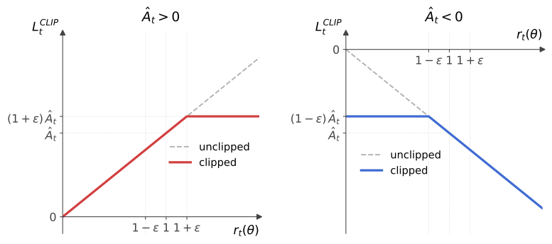
\[L^{\text{CLIP}}(\theta) = \mathbb{E}_{\tau\sim\pi_{\theta_{old}}}\Big[\smash{\sum_t} \min\big(r_t(\theta)\,\hat{A}_t\,,\, \text{clip}(r_t(\theta),\, 1-\varepsilon,\, 1+\varepsilon)\,\hat{A}_t\,\big)\Big]\]where $\text{clip}(r_t(\theta), 1-\varepsilon, 1+\varepsilon)$ caps the ratio into the interval $[1-\varepsilon,\, 1+\varepsilon]$:
\[\text{clip}(r_t(\theta),\, 1-\varepsilon,\, 1+\varepsilon) = \begin{cases} \,1-\varepsilon \quad & r_t(\theta) < 1-\varepsilon\\[2pt] \,r_t(\theta) & r_t(\theta)\in[1-\varepsilon,\, 1+\varepsilon]\\[2pt] \,1+\varepsilon & r_t(\theta) > 1+\varepsilon \end{cases}\]For clarity, let us write the per sample contribution, $L_t^{\text{CLIP}}(\theta)$, with its piecewise definition:
\[L_t^{\mathrm{CLIP}}(\theta)= \begin{cases} \,r_t(\theta)\,\smash{\hat A}_t \qquad& \smash{\hat A}_t>0 &r_t(\theta)\leq 1+\varepsilon\\[2pt] \,(1+\varepsilon)\,\smash{\hat A}_t & \smash{\hat A}_t>0 &r_t(\theta)>1+\varepsilon\\[2pt] \,r_t(\theta)\,\smash{\hat A}_t & \smash{\hat A}_t<0 &r_t(\theta)\geq 1-\varepsilon\\[2pt] \,(1-\varepsilon)\,\smash{\hat A}_t & \smash{\hat A}_t<0 \; &r_t(\theta)<1-\varepsilon \end{cases}\]The branches are easier to understand if we first recall what $\smash{\hat{A}}_t$ means. If $\smash{\hat{A}}_t >0$, the sampled action performed better than the critic expected, and increasing its probability improves the surrogate objective. If $\smash{\hat{A}}_t<0$, the action performed worse than expected, and decreasing its probability improves the objective. The ratio then measures how much of that change the new policy has already made. A ratio \(r_t=1.1\) means that the sampled action is now $10\%$ more likely than under the policy that collected it, \(r_t=0.8\) means that it is $20\%$ less likely.
Suppose first that the advantage is positive. While \(r_t \leq 1+\varepsilon\), PPO rewards increasing the probability of a good action. Beyond $1+\varepsilon$, the sample becomes flat, so making it even more likely earns no additional rewards. If the new policy already makes a good action much more likely than the old policy, PPO stops increasing its probability based on the current sample.
For a negative advantage the useful direction is reversed. PPO allows the probability of the bad action to decrease until \(r_t=1-\varepsilon\). Below that boundary, the sample again becomes flat. If the new policy already makes a bad action much less likely than the old policy, PPO stops decreasing its probability based on the current sample.
Everything so far concerns the actor, but the actor does not run on its own. The advantages that drive the clipped objective come from GAE, a discounted sum of TD errors, which exist only if something is estimating $V_\pi(s)$. In A$2$C, the critic was updated at every step, with its own parameters $w$ and its own learning rate \(\alpha_w\):
\[w \leftarrow w + \alpha_w \,\nabla_w V_w (s_t) \, \delta_t\]and each update aimed at the one step target \(r_{t+1} + \gamma V_w(s_{t+1})\). PPO, instead, waits until the whole batch of experience has been collected, and then fits the critic to it, as a regression. In this setup, three things change.
-
The target uses more information. The target for the critic is the estimate of the return from $s_t$, and GAE already produces one, at no extra cost. The advantage estimate is, by construction, the difference between two quantities: how good the trajectory turned out to be from $s_t$ onward, and how good the critic had predicted it would be.
\[\hat{A}_t = \big(\,\text{value of } s_t \text{ observed in the data}\,\big) - V_{old}(s_t)\]The first of the two is exactly the number we are looking for:
\[V_t^{\text{targ}} = \hat{A}_t + V_{old}(s_t)\] -
The target does not move. It is computed once, before the updates begin, and then stays fixed for all the epochs. In A$2$C the target changed together with the critic at every step.
-
There is a single set of parameters. The actor and the critic share most of their weights, usually there is one convolutional body with two small heads on top. Both depend on the same $\theta$ and are updated by the same optimizer, with the coefficient \(c_1\) deciding how much the value error counts against the policy term.
There is a need for a further term. Nothing so far rewards the policy for keeping its options open: the clipped objective pays for raising the probability of the actions that did well, and the value loss only concerns the critic. Left to itself, the actor drifts towards a deterministic policy. The clip does not prevent this. It limits how far the policy can move away from \(\pi_{\theta_{old}}\) within a single update, but once the batch is discarded and \(\theta_{old} \leftarrow \theta\), the new policy becomes the new reference. Every batch is free to move another $\varepsilon$ from wherever the previous one stopped, and after enough batches a probability can walk all the way to $1$.
For a policy method, this matters more than it would for a value method. Q-learning could be given an $\varepsilon$-greedy rule on top of its estimates, exploring regardless of what the values say. Here the only source of exploration is the randomness of the policy itself. If \(\pi_\theta(a \vert s)\) is close to $1$, the other actions are almost never sampled. If they are never sampled, no advantage is computed for them, and with no advantage there is nothing that can push their probability back up. If the policy settles on the wrong action early, nothing later fixes it.
The entropy of the action distribution measures how spread out it is:
\[S[\pi_\theta](s) = -\sum_a \pi_\theta(a|s)\,\log \pi_\theta(a|s)\]It is largest when the policy is undecided and zero when it is deterministic. With two actions, \((0.5,\,0.5)\) gives $\log 2 \approx 0.69$, while \((0.9,\,0.1)\) gives $0.33$ and \((0.99,\,0.01)\) gives $0.06$.
Adding \(c_2\,S[\pi_\theta](s_t)\) to an objective that is maximized pays the policy for staying undecided, so that becoming confident costs something. An action has to earn its probability with an advantage large enough to outweigh the entropy lost. It is meant to keep the policy from settling on one action before the advantages are reliable, not to stop it from ever settling.
All of the terms combine into a single objective to maximize:
\[L(\theta) = \mathbb{E}_{\tau\sim\pi_{\theta_{old}}}\Big[\sum_t \, L_t^{\text{CLIP}}(\theta) \,-\, c_1 \underbrace{\big(V_\theta(s_t) - V_t^{\text{targ}}\big)^2\\[4pt]}_{\text{value function loss}} \,+\, c_2 \underbrace{S\big[\pi_\theta\big](s_t)\\[4pt]}_{\text{entropy bonus}}\,\Big]\]with typical coefficients $c_1 = 0.5$ and $c_2 \approx 0.01$. Every term inside the sum has a role:
- $L_t^{\text{CLIP}}$ improves the policy while limiting the incentive for large probability changes
- the squared error trains the critic towards $V_t^{\text{targ}}$ (subtracted, since it’s maximized)
- the entropy bonus rewards a broad action distribution and preserves exploration
- Initialize actor-critic parameters $\theta$
- Initialize $\alpha$, $\gamma$, $\lambda$, $\varepsilon$, $c_1$, $c_2$
- Repeat until convergence:
- Run $\pi_{\theta_{old}}$ for $T$ steps, storing $(s_t,\, a_t,\, r_{t+1},\, \log \pi_{\theta_{old}}(a_t|s_t),\, V(s_t))$
- Compute advantages $\smash{\hat{A}}_t$ with GAE and value targets $V_t^{\text{targ}} = \smash{\hat{A}}_t + V(s_t)$
- For $K$ epochs:
- Split the collected steps into minibatches
- For each minibatch, update $\theta$ by gradient ascent on
$$L(\theta) = \textstyle\sum_t\, L_t^{\text{CLIP}}(\theta) - c_1 (V_\theta(s_t) - V^{\text{targ}}_t)^2 + c_2\, S[\pi_\theta](s_t)$$
- Update $\theta_{old} \leftarrow \theta$, discard the collected steps
- Return the learned policy $\pi_\theta$
Let us conclude with the usual small example, following one PPO policy update. There are two states, \(S = \{\text{low}, \text{high}\}\), and two actions, \(A = \{x,y\}\). The actor stores one preference \(\theta_{s,a}\) for every state-action pair, turned into probabilities by a softmax:
\[\pi_\theta(x|s)=\frac{e^{\theta_{s,x}}} {e^{\theta_{s,x}}+e^{\theta_{s,y}}} \qquad \pi_\theta(y|s)=\frac{e^{\theta_{s,y}}} {e^{\theta_{s,x}}+e^{\theta_{s,y}}}\]As in A$2$C’s example, a single step moves both preferences of a state by the same amount and in opposite directions, so $\theta_{s,y} = -\theta_{s,x}$ at every step.
Before collecting any data, all preferences are zero. The policy chooses either action with probability $0.5$ at any state. This policy is saved as \(\pi_{\theta_{old}}\) and used to generate two episodes:
\[\begin{align} \text{episode }1: \quad &(\text{low}, x) \xrightarrow{+1} (\text{high}, y) \xrightarrow{+5} \text{ terminal}\\[0pt] \text{episode }2: \quad &(\text{low}, y) \xrightarrow{+2} \text{ terminal} \end{align}\]Set $\gamma=1$, so future rewards are not discounted. In the first episode, the return from $\text{low}$ is $1+5=6$, while the return from $\text{high}$ is $5$. In the second episode, the return from $\text{low}$ is $2$. Suppose that the old critic is still imperfect and predicts:
\[V_{\pi_{old}}(\text{low})=3\, \qquad V_{\pi_{old}}(\text{high})=4\,\]Set $\lambda=1$. At this end of GAE the advantage of a sample is its return minus the old critic prediction, and the target the critic is fitted to is the return itself. Both are computed once and kept fixed for all $K$ epochs:
\(\begin{array}{lll} \quad\mathrel{\raise 1pt\hbox{$\scriptsize\bullet$}} \normalsize\,\, (\text{low}, x): & \; \smash{\hat{A}}_t = 6 - 3 = +3\, & \; V_t^{\text{targ}} = 6\\[-2pt] \quad\mathrel{\raise 1pt\hbox{$\scriptsize\bullet$}} \normalsize\,\, (\text{high}, y): & \; \smash{\hat{A}}_t = 5 - 4 = +1\, & \; V_t^{\text{targ}} = 5\\[-2pt] \quad\mathrel{\raise 1pt\hbox{$\scriptsize\bullet$}} \normalsize\,\, (\text{low}, y): & \; \smash{\hat{A}}_t = 2 - 3 = -1\, & \; V_t^{\text{targ}} = 2 \end{array}\)
The formula \(V_t^{\text{targ}} = \hat{A}_t + V_{\pi_{old}}(s_t)\) introduced earlier returns these exact three numbers, since adding the prediction back cancels the subtraction. The actor has two independent probabilities to update:
\[p=\pi_\theta(x|\text{low})\, \qquad q=\pi_\theta(y|\text{high})\]The other probabilities are $1-p$ and $1-q$. Since every action had probability $0.5$ under the old policy, the three ratios are:
\[r_{\text{low},x}=\frac{p}{0.5}\, \qquad r_{\text{low},y}=\frac{1-p}{0.5}\, \qquad r_{\text{high},y}=\frac{q}{0.5}\]Set $\varepsilon=0.2$. The clipping interval is $[0.8,1.2]$. At $p=0.6$, the good action $x$ in $\text{low}$ reaches the upper boundary and the bad action $y$ reaches the lower one:
\[\frac{0.6}{0.5}=1.2\, \qquad \frac{1-0.6}{0.5}=0.8\]The positive-advantage action $y$ in $\text{high}$ reaches its upper boundary when $q=0.6$ as well. The two policy contributions are therefore:
\[\begin{align} L_{\text{low}\phantom{\text{l}}}^{\text{CLIP}}(p) &= \begin{cases} \textstyle\frac{p}{0.5}\,(+3)+\frac{1-p}{0.5}\,(-1)=8p-2 \quad &p\leq0.6\\[2pt] 1.2\,(+3)+0.8\,(-1)=2.8 &p>0.6 \end{cases}\\[4pt] L_{\text{high}}^{\text{CLIP}}(q) &= \begin{cases} \rlap{\textstyle\frac{q}{0.5}\,(+1)=2q}\phantom{\frac{p}{0.5}\,(+3)+\frac{1-p}{0.5}\,(-1)=8p-2} \quad &q\leq0.6\\[2pt] 1.2\,(+1)=1.2 &q>0.6 \end{cases} \end{align}\]Let us now include the critic and entropy. Let \(v_l=V_\theta(\text{low})\) and \(v_h=V_\theta(\text{high})\). At the start they equal the saved predictions, $v_l=3$ and $v_h=4$. In this example the policy preferences and the two values are separate entries, but together they play the role of the actor-critic parameters $\theta$. A neural implementation would update its shared weights through the same objective. For the two actions, let us (re-)define the entropy:
\[H(z)=-z\log z-(1-z)\log(1-z)\,.\]Summing over the three stored steps, as the objective above does, and taking $c_1=0.5$ and $c_2=0.01$, the complete objective is:
\[L= \underbrace{L_{\text{low}}^{\text{CLIP}}(p) +L_{\text{high}}^{\text{CLIP}}(q)}_{\text{actor}} - 0.5 \underbrace{\big[(v_l-6)^2+(v_h-5)^2+(v_l-2)^2\big]}_{\text{critic}} + 0.01\underbrace{\big[2H(p)+H(q)\big]}_{\text{entropy}}\]The value $2$ before $H(p)$ is there because $\text{low}$ appears twice in the data, while $\text{high}$ appears once. As before, PPO updates preferences, not directly probabilities. There are four values to update, $\theta_{\text{low},x}$, $\theta_{\text{high},y}$, $v_l$ and $v_h$, so we need a gradient of $L$ for each. The two remaining preferences follow by symmetry, $\theta_{\text{low},y} = -\theta_{\text{low},x}$ and $\theta_{\text{high},x} = -\theta_{\text{high},y}$.
Take $\theta_{\text{low},x}$ first. Only two terms of $L$ depend on it, the low-state policy term and the low-state entropy, and both reach it through $p$. The chain rule splits the work in two parts: how much $L$ changes when $p$ changes, and how much $p$ changes when the preference changes. The second factor is the softmax derivative:
\[\frac{\partial p}{\partial \theta_{\text{low},x}} = p\,(1-p)\]For the first factor, take $p\leq0.6$, so that nothing is clipped yet. There the policy term is $8p-2$, whose slope is the constant $8$, and the entropy term is $0.02\,H(p)$, whose slope is:
\[0.02\,H'(p) = 0.02\,\log\Big(\frac{1-p}{p}\Big)\]Multiplying the two factors gives the gradient for $\theta_{\text{low},x}$, and the same reasoning applied to $\text{high}$, where the policy term is $2q$ and the entropy carries $0.01$ because the state appears once, gives the gradient for $\theta_{\text{high},y}$:
\[\begin{aligned} \frac{\partial L}{\partial\theta_{\text{low},x}} = \frac{\partial L}{\partial p}\,\frac{\partial p}{\partial \theta_{\text{low},x}} &=\Big[8+0.02\log\Big(\frac{1-p}{p}\Big)\Big] \,p\,(1-p)\\[2pt] \frac{\partial L}{\partial\theta_{\text{high},y}} = \frac{\partial L}{\partial q}\,\frac{\partial q}{\partial \theta_{\text{high},y}} &=\Big[2+0.01\log\Big(\frac{1-q}{q}\Big)\Big] \,q\,(1-q) \end{aligned}\]The two values are easier: each appears only in the critic group, where the derivative of a squared residual is twice that residual, and the $0.5$ in $c_1$ cancels the $2$:
\[\begin{aligned} \frac{\partial L}{\partial v_l} &=-[(v_l-6)+(v_l-2)]=8-2v_l\\[2pt] \frac{\partial L}{\partial v_h} &=-(v_h-5)=5-v_h. \end{aligned}\]The state $\text{low}$ contributes two residuals because it was visited twice, and they pull its value towards their average, $4$. The state $\text{high}$ contributes one, pulling its value towards $5$.
Let $\alpha=0.05$. In the first epoch, $p=q=0.5$, so no policy term is clipped and both entropy gradients are zero (since it becomes $\log(1)$):
\[\begin{aligned} \theta_{\text{low},x}&\leftarrow 0+0.05\,[\,8\cdot0.5\,(1-0.5)\,]=0.100\\[2pt] \theta_{\text{high},y}&\leftarrow 0+0.05\,[\,2\cdot0.5\,(1-0.5)\,]=0.025\\[2pt] v_l&\leftarrow3+0.05\,(8-2\cdot3)=3.100\\[2pt] v_h&\leftarrow4+0.05\,(5-4)=4.050 \end{aligned}\]This is one complete PPO update: the policy makes the advantageous actions more likely, the critic moves towards the fixed value targets, and entropy is present but contributes zero because the policy begins perfectly balanced. Repeating the same calculation for four epochs gives:
| After epoch | $\quad{\text{low} \;(\theta_{\text{low},x}, \,p)}\quad$ | $\quad{\text{high} \;(\theta_{\text{high},y}, \,q)}\quad$ | ${v_l}$ | ${v_h}$ |
|---|---|---|---|---|
| $1$ | $(0.100,\,0.550)$ | $(0.025,\,0.512)$ | $3.100$ | $4.050$ |
| $2$ | $(0.199,\,0.598)$ | $(0.050,\,0.525)$ | $3.190$ | $4.098$ |
| $3$ | $(0.295,\,0.643)$ | $(0.075,\,0.537)$ | $3.271$ | $4.143$ |
| $4$ | $(0.295,\,0.643)$ | $(0.100,\,0.550)$ | $3.344$ | $4.185$ |
At the start of epoch 3, $p\approx0.598$ is still below the clipping point, so the policy gradient carries it slightly past the boundary to $0.643$. In epoch 4, the low-state policy term is flat: it contributes no gradient because both of its useful changes are clipped. The entropy term still contributes a very small negative gradient, changing \(\theta_{\text{low},x}\) from $0.295005$ to $0.294870$ and moving $p$ from $0.643368$ to $0.643305$. The rounded displays both as $0.295$ and $0.643$.
The other parts of the update continue. Since $q$ has not reached $0.6$, the high-state policy still raises it. The critic also keeps moving $v_l$ towards $4$ and $v_h$ towards $5$. After the chosen $K=4$ epochs, PPO saves the updated policy as the next \(\pi_{\theta_{old}}\), discards these samples, and collects new data. Clipping has limited what the old data can do to $p$ without preventing the critic, entropy, or the still-unclipped part of the policy from being updated.
Reinforcement Learning Saga — Part II: From Q-learning to PPO
- Tabular Q-learning update (Part I)
\(\\[2pt] \rule{0pt}{10pt} \qquad Q_\pi(s,a) \leftarrow Q_\pi(s,a) + \alpha\,(r + \gamma\, \textstyle{\max_{a'}}\, Q_\pi(s',a') - Q_\pi(s,a))\)
$\boldsymbol{\downarrow}$ a table cannot represent a screen of pixels\(\\[8pt]\) - DQN loss
\(\\[2pt] \rule{0pt}{8pt} \qquad L(\theta) = \mathbb{E}\big[\big(r + \gamma\, \textstyle{\max_{a'}}\, Q_{\theta^-}(s',a') - Q_\theta(s,a)\big)^2\big]\)
$\boldsymbol{\downarrow}$ the policy is still an argmax over actions, values remain a proxy for behavior\(\\[8pt]\) - Policy objective, maximized by ascent
\(\\[6pt] \rule{0pt}{10pt} \qquad \theta \leftarrow \theta + \alpha\,\nabla_\theta J(\theta)\)
\(\\[4pt]\qquad J(\theta) = \mathbb{E}_{\tau\sim\pi_\theta}[G(\tau)]\)
$\boldsymbol{\downarrow}$ the gradient appears to depend on the unknown dynamics of the environment\(\\[8pt]\) - Policy gradient theorem
\(\\[2pt] \rule{0pt}{10pt} \qquad \nabla_\theta J(\theta) = \mathbb{E}_{\tau\sim\pi_\theta}\big[\textstyle{\sum_t}\, \nabla_\theta \log \pi_\theta(a_t \hspace{-2pt} \mid \hspace{-2pt} s_t)\; G_t\big]\)
$\boldsymbol{\downarrow}$ the absolute scale of rewards is not what distinguishes good actions\(\\[8pt]\) - Baseline and advantage
\(\\[6pt] \rule{0pt}{10pt} \qquad \nabla_\theta J(\theta) = \mathbb{E}_{\tau\sim\pi_\theta}\big[\textstyle{\sum_t}\, \nabla_\theta \log \pi_\theta(a_t \hspace{-2pt}\mid\hspace{-2pt} s_t)\,\big(G_t - b(s_t)\big)\big], \,\, b = V_\pi(s_t)\)
\(\\[4pt] \qquad A_\pi(s,a) = Q_\pi(s,a) - V_\pi(s)\)
$\boldsymbol{\downarrow}$ the true advantage is unknown, it must be learned\(\\[8pt]\) - One step advantage estimate, the TD error
\(\\[2pt] \qquad \rule{0pt}{10pt} \hat{A}_t^{(1)} = \delta_t = r_{t+1} + \gamma\,V_w(s_{t+1}) - V_w(s_t)\)
$\boldsymbol{\downarrow}$ the same error can update both the policy and the value estimate\(\\[8pt]\) - A$2$C
\(\\[6pt] \rule{0pt}{10pt} \qquad \theta \leftarrow \theta + \alpha_\theta\, \delta_t\, \nabla_\theta \log \pi_\theta(a_t \mid s_t)\)
\(\\[4pt] \qquad w \leftarrow w + \alpha_w\, \delta_t\, \nabla_w V_w(s_t)\)
$\boldsymbol{\downarrow}$ one step is biased, Monte Carlo carries the noise of the whole episode\(\\[8pt]\) - GAE
\(\\[3pt] \qquad \hat{A}_t^{\,GAE \,(\gamma,\,\lambda)} = \textstyle{\sum}_{\ell\,\geq\,0} (\gamma\lambda)^{\ell}\, \delta_{t+\ell}\)
$\boldsymbol{\downarrow}$ the update direction is useful, but after one update the data belongs to the old policy\(\\[8pt]\) - Importance sampling
\(\\[6pt] \rule{0pt}{12pt} \qquad r_t(\theta) = \frac{\pi_\theta(a_t \mid s_t)}{\pi_{\theta_{old}}(a_t \mid s_t)}\)
\(\\[4pt]\qquad L(\theta) = \mathbb{E}_{\tau\sim\pi_{\theta_{old}}}\big[\textstyle{\sum_t}\, r_t(\theta)\,\hat{A}_t\big]\)
$\boldsymbol{\downarrow}$ the correction is reliable only while the new policy remains close to the old one\(\\[8pt]\) - TRPO
\(\\[2pt] \qquad \max_\theta\, \mathbb{E}_{\tau\sim\pi_{\theta_{old}}}\big[\textstyle{\sum_t}\, r_t(\theta)\,\hat{A}_t\big] \;\text{ s.t.}\; \mathbb{E}\big[\text{KL}(\pi_{\theta_{old}}(\cdot \hspace{-2pt}\mid\hspace{-2pt} s_t) \,\Vert\, \pi_\theta(\cdot \hspace{-2pt}\mid\hspace{-2pt} s_t))\big] \leq \delta\)
$\boldsymbol{\downarrow}$ enforcing the constraint requires expensive second-order optimization\(\\[8pt]\) - PPO
\(\\[6pt] \qquad L^{\text{CLIP}}(\theta) = \mathbb{E}_{\tau\sim\pi_{\theta_{old}}}\big[\textstyle{\sum_t} \min\big(r_t(\theta)\,\hat{A}_t,\; \text{clip}(r_t(\theta), 1\!-\!\varepsilon, 1\!+\!\varepsilon)\,\hat{A}_t\big)\big]\)
\(\\[8pt] \qquad L(\theta) = \mathbb{E}_{\tau\sim\pi_{\theta_{old}}}\big[\textstyle{\sum_t}\, L_t^{\text{CLIP}}(\theta) - c_1 \big(V_\theta(s_t) - V_t^{\text{targ}}\big)^2 + c_2\, S[\pi_\theta](s_t)\big]\)